TensorFlow for Foreign Exchange Market: Analyzing Time-Series Data

Latent variable models
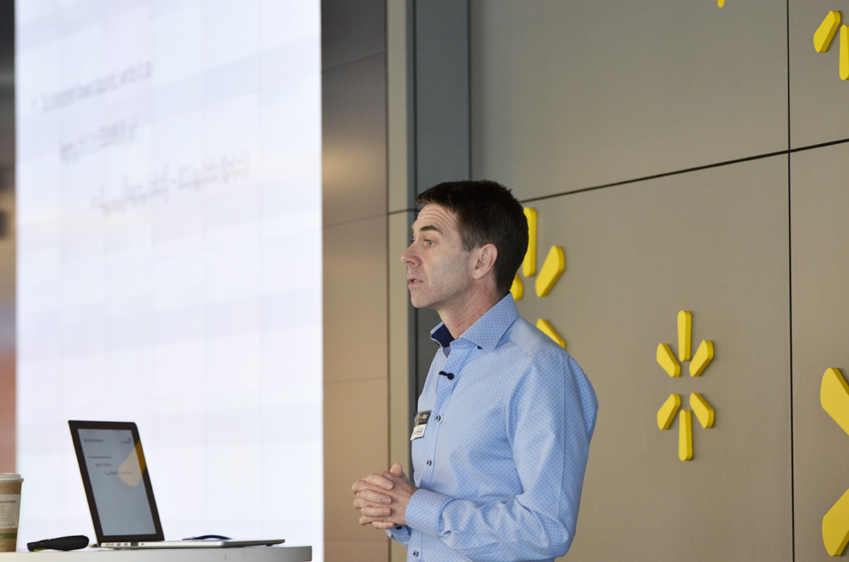
During TensorBeat 2017, Daniel Egloff looked into the value brought by deep learning solutions to the financial sector. He shared his experience of building a generative model for financial time-series data and demonstrated how to implement it with TensorFlow. Daniel noted that this kind of models—for example, generative adversarial networks (GANs) or variational autoencoders (VAEs)—is quite a recent innovation in deep learning.
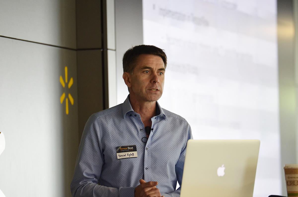
“In finance, deep learning is complementary to the existing models, not a replacement.”
—Daniel Egloff, QuantAlea
So, how does deep learning bring value to finance?
- Richer functional relationship between explanatory and response variables
- Model complicated interactions
- Automatic feature discovery
- Capable to handle large amounts of data
- Standard training procedures with backpropagation and stochastic gradient descent
- A variety of frameworks and tooling
In this context, Daniel overviewed latent variable models, which allow to:
- Better explain data distribution
- Postulate prior distribution
- Define the likelihood of data as a latent variable function
- Infer distribution of latent variable given data
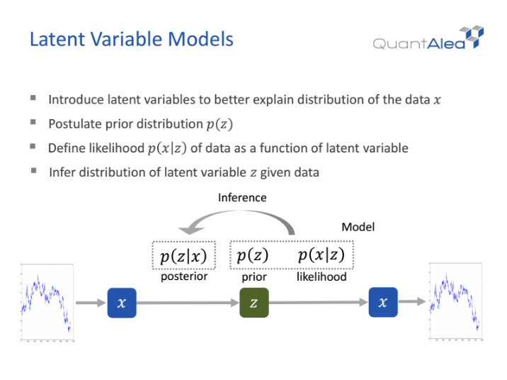
A latent variable can be thought of as an encoded representation, where the likelihood serves as a decoder and a posterior as an encoder.
Dealing with maximum likelihood, one may face that a marginal and a posterior are intractable and their calculation suffers from exponential complexity. This can be addressed with Markov chain, Hamiltonian Monte Carlo algorithm, and approximation/variational inference.
To enable approximation with variational autoencoders:
- Assume latent space with prior distribution
- Parameterize the likelihood with a deep neural network
- Approximate intractable posterior with a deep neural network
- Learn the parameters with backpropagation
When applying it to time-series data, Daniel employed the Gaussian function, its distributions (the parameters are calculated from a recurrent neural network), and variational inference (to train a model). When embedding time-series data, he used a lag of 20 to 60 historical observations at each time step.
Implementation with TensorFlow
To run the process of training a TensorFlow-based model, P100 GPUs were chosen. (However, long time-series and large batch sizes require substantial GPU memory. We’ve previously written how to tackle such a problem.)
So, to unroll a recurrent neural network (RNN), tf.nn.dynamic_rnn may be used as it is simple to work with and handles variable sequence length. Though, it is not flexible enough for generative networks. To enjoy more flexibility, one may use tf.while_loop. Still, it comes in more coding and requires a comprehensive understanding of control structures.
Daniel then demonstrated the implementation at the code level, which comprises the following steps:
- Variable and weight setup
- Allocation of TensorArray objects
- Filling input TensorArray objects with data
- While loop body inference (updating the inference RNN state and the generator RNN state)
- Calling a while loop
- Stacking TensorArray objects
- Loss calculation
The code samples are available in the slide deck below.
Analyzing FX market data
How is it applicable to real-life needs of the financial sector? Daniel demonstrated how deep learning can help out foreign exchange (FX) market.
Operating 24 hours, five and a half days a week, the world’s largest and most liquid market is a perpetual fierce competition between the participants. The FX market is decentralized, which means there is no need to go through a centralized exchange and a price for a particular currency can change any second. The market’s daily turnover is equal to $5.1 trillion in 2016, with the peak turnover registered in 2013—$5.3 trillion, which is a bit more than $220 billion per hour.
With a humongous data flow, a common practice Daniel shared is collecting tick data of the overlapping US and European session. The reason for that is simple as the trading activity is the highest, offering valuable data sources to drive insights from. So, the model is trained on this fresh data captured and is further applied to the rest of the US session.
Daniel then showed a 10-minute data flow sampled and aggregated in an open-high-low-close chart.
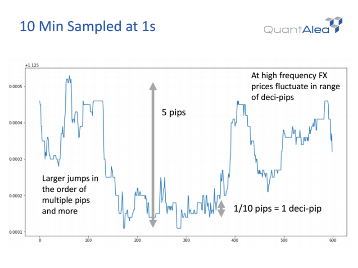
As can be seen, there are quite big jumps in price moves in the chart. To get value out of this info, one may normalize data with the standard deviation over a training interval. In 2016, there were 260 trading days, and the team trained a model per day.
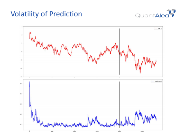
Thus, the solution helps to track the pace the FX market moves at, analyze peak vs. recession times, observe the trends, and make predictions based on this information.
Want details? Watch the video!
Related slides
Further reading
- TensorFlow in Finance: Discussing Predictive Analytics and Budget Planning
- Learning Financial Data and Recognizing Images with TensorFlow and Neural Networks
- Performance of Distributed TensorFlow: A Multi-Node and Multi-GPU Configuration
About the expert
Daniel Egloff is a partner at InCube Group and Managing Director of QuantAlea, a Swiss software engineering company specialized in GPU software development. He studied mathematics, theoretical physics, and computer science. Daniel has 15+ years of experience as a quant in the financial service industry.